PypeIt QA
As part of the standard reduction, PypeIt generates a series of Quality Assurance (QA) files. This documentation describes the typical outputs, in the typical order that they appear. The basic arrangement is that individual PNG files are created and then a set of HTML files are generated to organize viewing of the PNGs.
HTML
When the code completes (or crashes out), a set of HTML files are generated in the QA/ folder. There is one HTML file per MasterFrame set and one HTML file per science exposure. Example names are MF_A_01_aa.html and J124_J1247-0337_LRISr_2017Mar20T140044.html.
Quick links are provided to allow one to jump between the various files.
Calibration QA
The first QA PNG files generated are related to calibration processing. There is a unique one generated for each setup and detector and (possibly) calibration set.
Generally, the title describes the type of QA and the sub-title indicates the user who ran PypeIt and the date of the processing.
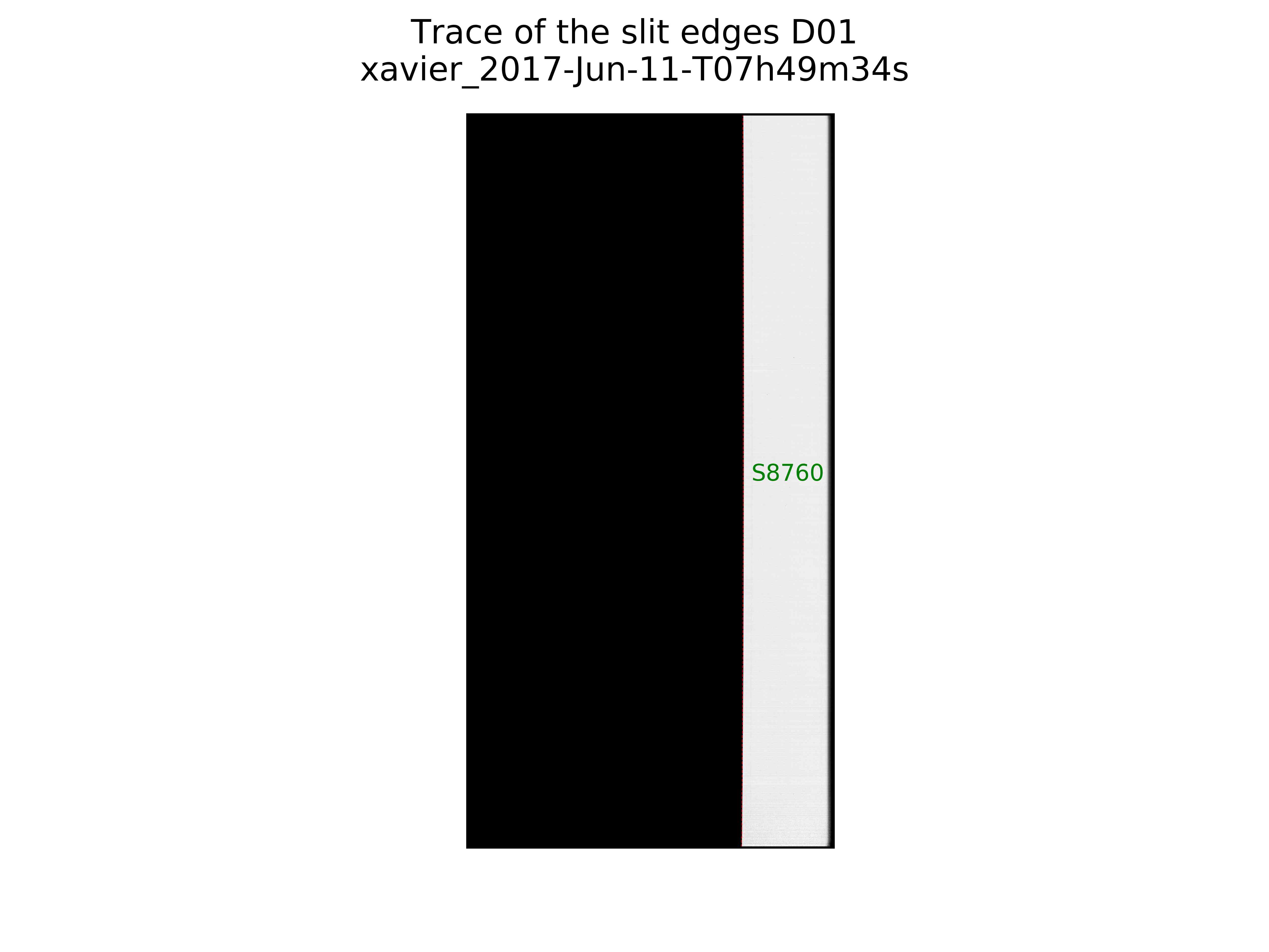
Slit Edge QA
The first output is a plot showing the flat image of the given detector. The left/right slit edges are marked with red/cyan dashed lines. The slit name is labelled in green and the number indicates the position of the slit center on the detector mapped to the range [0-10000]. Here is an example:
Blaze QA
This page shows the blaze function measured from a flat-field image, and the fit to this function. There should be good correspondence between the two. Here is an example:
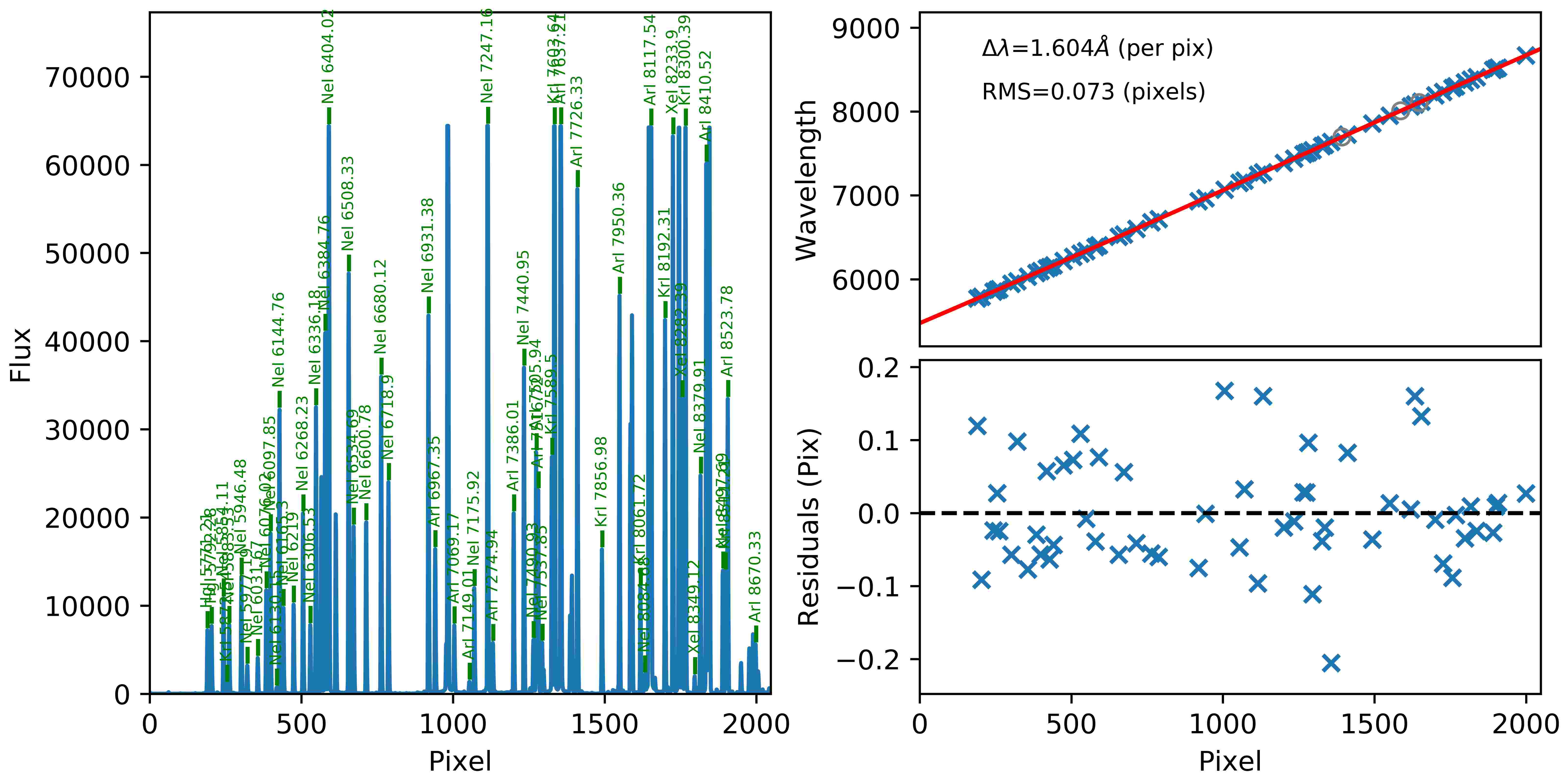
Wavelength Fit QA
This page shows the arc spectrum with labelled arc lines in the left panel and the fit and residuals to the fit in the right panels. Good solutions should have RMS < 0.1 pixels. Here is an example:
Spectral Tilts QA
There are generally a series of PNG files describing the analysis of the tilts of the arc lines.
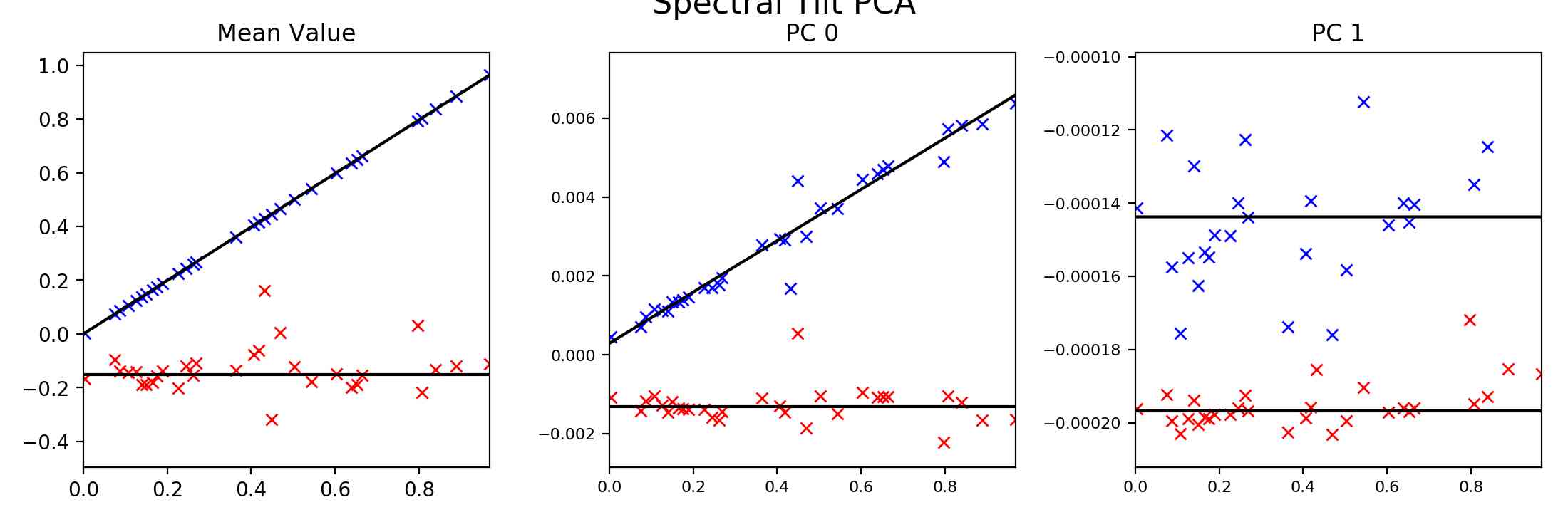
Arc Tilt PCA
One page should show fits to the PCA components describing the arcline tilt fits. One hopes for good models to the data (blue crosses; red crosses indicate lines ignored in the analysis) in the first two panels, and that the values for PC1 are small. Here is an example:
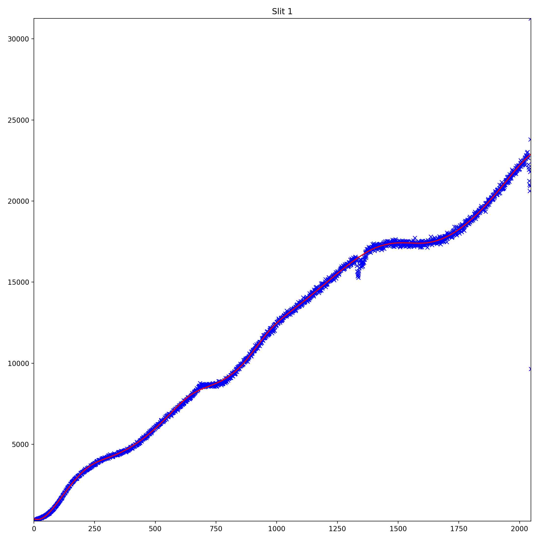
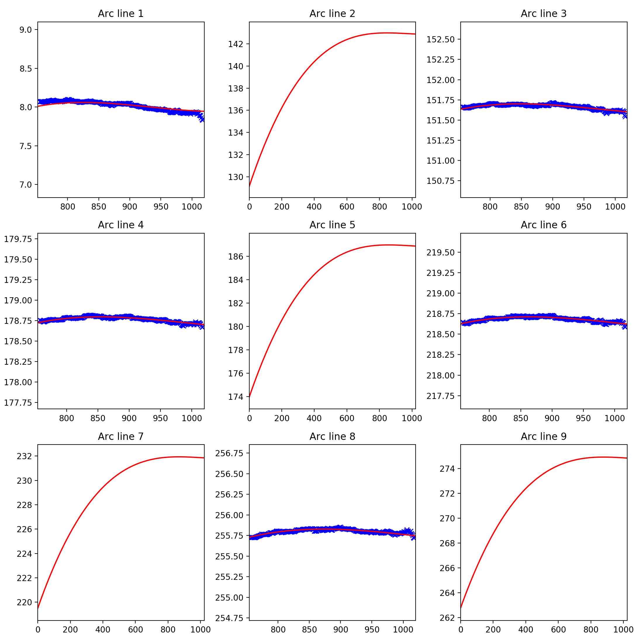
Arc Tilt Plots
There are then a series of PNG files showing the arc lines across the detector (blue) and associated fits (red). Here is an example page:
Exposure QA
For each processed, science exposure there are a series of PNGs generated, per detector and (sometimes) per slit.
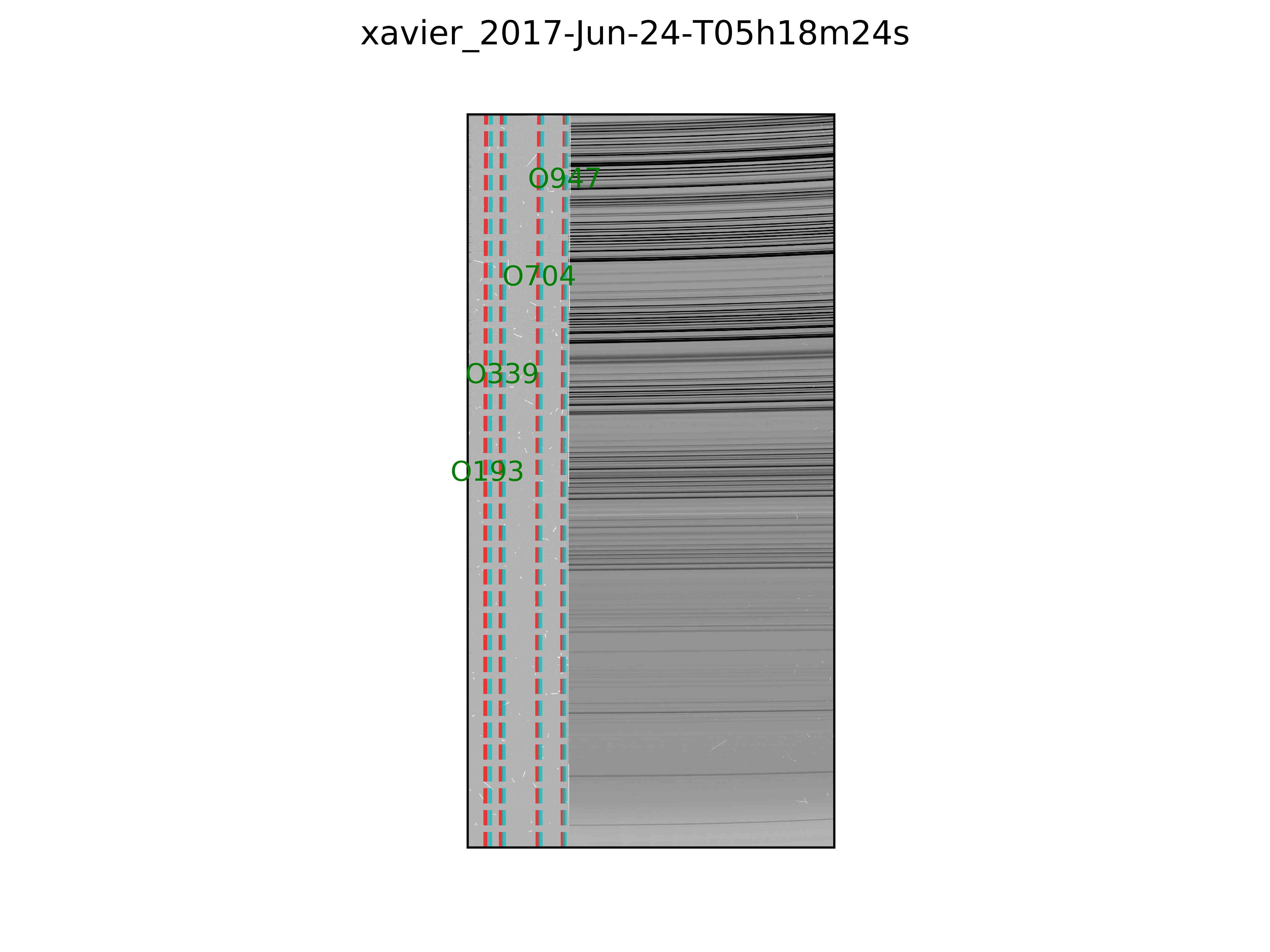
Object Trace QA
An image of the sky-subtracted slit is displayed. Overlayed are the left/right (red/cyan) edges of the extraction region for each object. These are also labeled by the object ID value where the 3-digit number is the trace position relative to the slit, ranging from 0-1000. Here is an example:
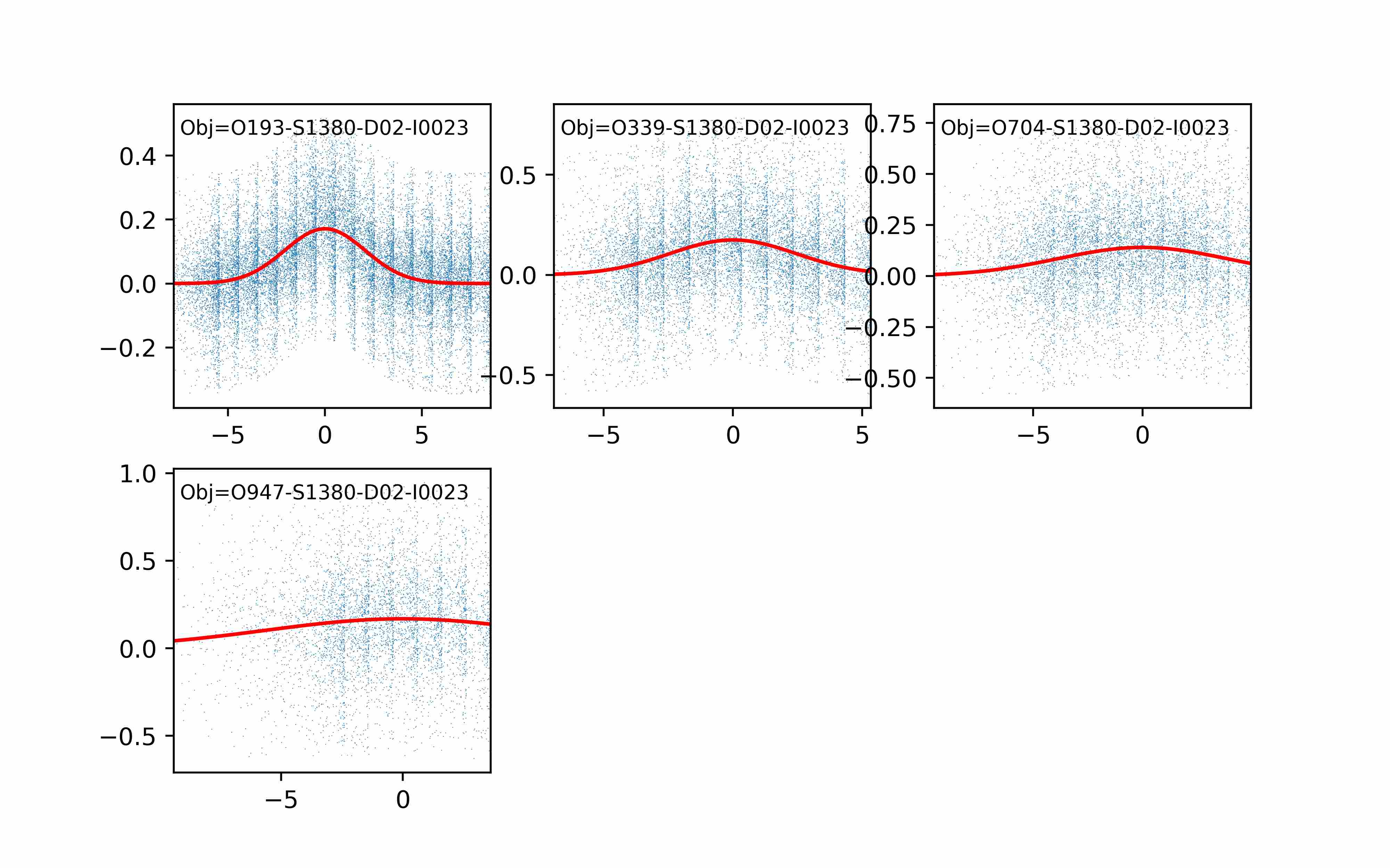
Object Profile QA
For all of the objects in a given slit where optimal extraction was performed the spatial profile and the fit are displayed. The x-axis is in units of pixels. Here is an example:
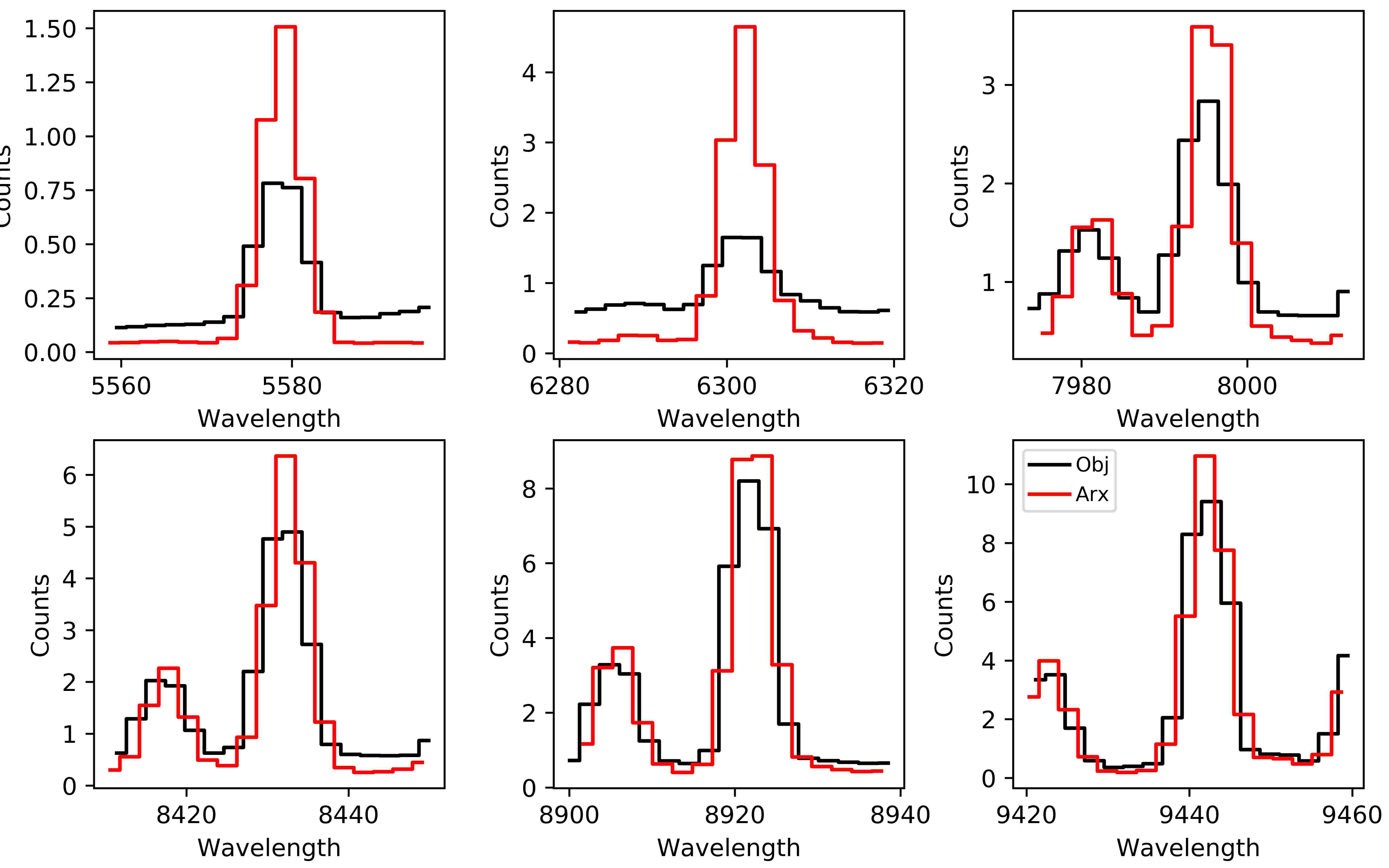
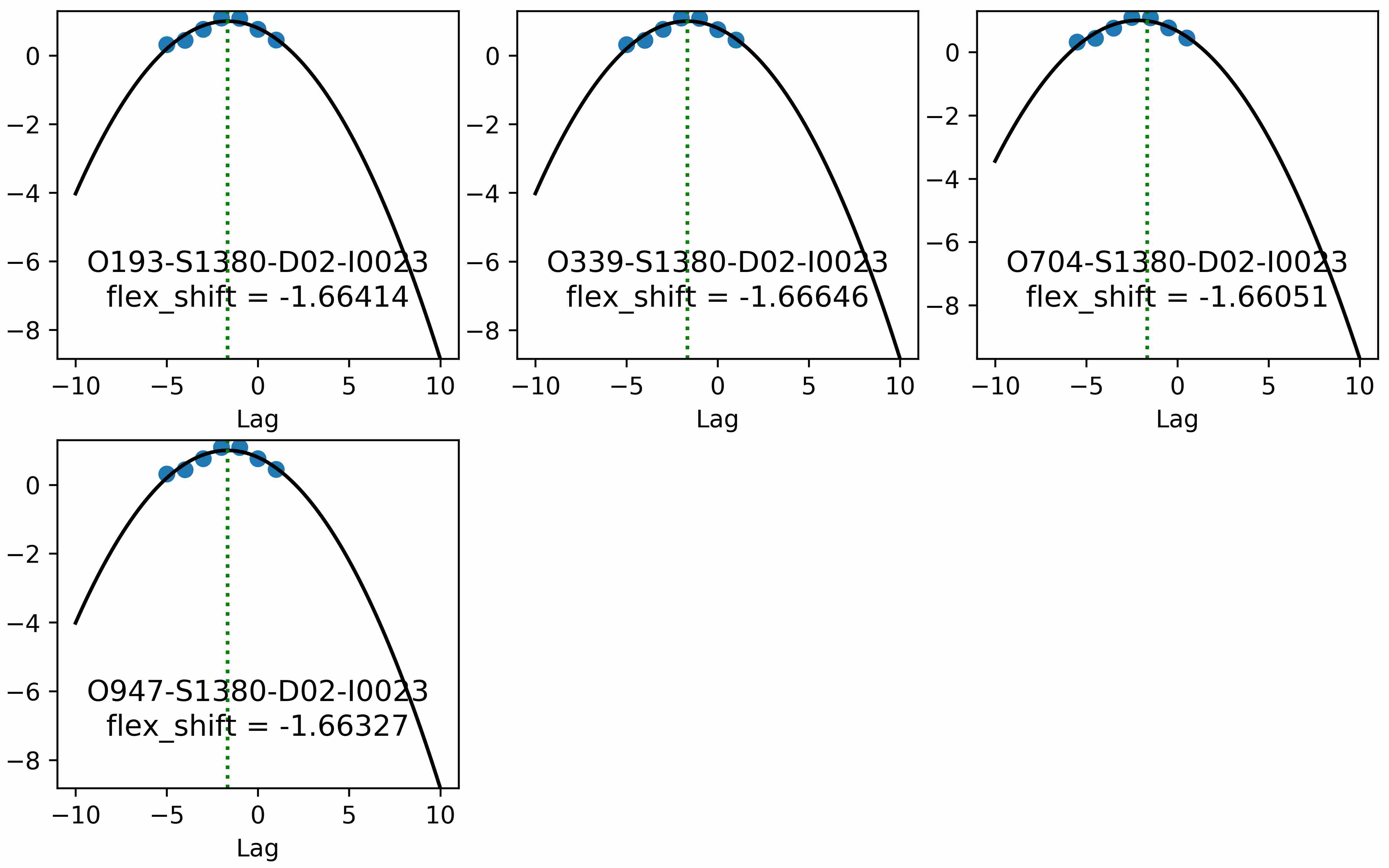
Flexure QA
If a flexure correction was performed (default), the fit to the correlation lags per object is shown and the adopted shift is listed. Here is an example:
There is then a plot showing several sky lines for the analysis of a single object (brightest) from the data compared against an archived sky spectrum. These should coincide well in wavelength. Here is an example: